Large language models get explained in jargon that assumes you already know the jargon. Attention, quantization, activations, LoRA: each term is defined using three others you also do not have yet, and the whole thing reads like a wall.
This is that wall taken apart. It starts smaller than the weights, at a single number, and adds one idea at a time, each built only on the ones before it. By the end, every term points at a concrete mechanism instead of another word. Nothing here assumes prior machine-learning knowledge, only patience for a definition to finish before the next one starts.
Two colors run through the diagrams. Amber marks values that are fixed after training, the learned weights. Teal marks values that are computed live from the input, the ones that exist only while the model is running. Keeping those two apart is half the battle, so the split is worth watching from the start.
The smallest piece: a number and its dtype
Strip an LLM all the way down and you reach a single number, usually a decimal like 0.0374 or -1.82. A model has billions of them. Everything else is machinery for storing those numbers and multiplying them together.
Before anything else, that number has a dtype, the data type it is stored as, which fixes how many bits it eats and how precise it can be:
FP32: 32-bit float, 4 bytes, very precise, the old training default.FP16/BF16: 16-bit, 2 bytes, the modern default.FP8: 8-bit, 1 byte, fast on newer GPUs.INT8/INT4: integer quantized values, used to shrink a model onto smaller hardware.
Fewer bits means a smaller file, less memory, faster math, and slightly less accuracy. Choosing a dtype is trading quality for footprint, and that trade turns out to matter enormously later.
Anatomy of a float. A floating-point number splits its bits three ways: a sign bit, some exponent bits that set the range (how large or small a value it can be), and some mantissa bits that set the precision (how many significant digits it carries).
| Format | Bits | Exponent | Mantissa | Max value | Significant digits |
|---|---|---|---|---|---|
| FP32 | 32 | 8 | 23 | ~3.4e38 | ~7 |
| FP16 | 16 | 5 | 10 | 65,504 | ~3 to 4 |
| BF16 | 16 | 8 | 7 | ~3.4e38 | ~2 to 3 |
The two 16-bit formats spend their bits differently. BF16 copies FP32's 8 exponent bits, so it keeps FP32's full range but is coarse. FP16 spends bits the other way: more precise, but a tiny maximum of 65,504. BF16 is not wider-range than FP32; it matches FP32's range and gives up precision to fit in half the memory.
Why this matters for training. The rule is that range errors are catastrophic and precision errors are just noise. During training, the signal that nudges each weight spans many orders of magnitude. In FP16's narrow range, large values overflow to infinity, then to NaN, and poison the whole model, while tiny values underflow to zero and stop learning. FP16 training only survives with a scaling hack; BF16, with FP32's range, needs none. Low precision, on the other hand, is tolerable, because training is a massively averaged, already-noisy process and rounding noise washes out. So real training runs in mixed precision: fast BF16 for the bulk of the math, with a master copy of the weights kept in FP32 so tiny updates accumulate faithfully instead of getting swamped.
Hold on to one line from this section: the dtype is a dial between quality and size, and low precision hurts far less than it looks like it should. That single fact reappears twice more before the end.
Grids of numbers: tensors, dims, and parameters
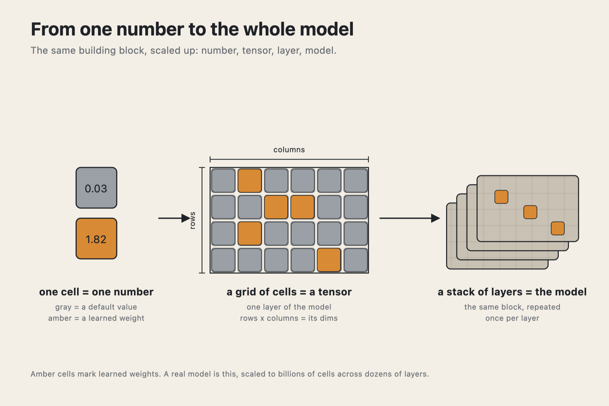
One number is not useful. Numbers become useful when they are arranged into grids.
A tensor is exactly that, a grid of numbers generalized to any number of dimensions:
- 0 dimensions is a single number (a scalar).
- 1 dimension is a list (a vector).
- 2 dimensions is a table (a matrix).
- 3 or more dimensions is a stack of tables, and onward.
Tensors are the universal unit of everything that follows. The weights are tensors. Your input, once converted to numbers, is a tensor. Every value moving through the model is a tensor, and every operation is math on tensors.
Two words that get tangled together are worth separating now. A scalar is a shape fact: a single number, a 0-dimensional tensor, which can be anything at all, an input value, a constant, or one entry pulled out of a grid. A parameter is a role fact: a number the training learned, a weight or a bias. Every parameter is a single number, but not every number is a parameter. The distinction is between "how many dimensions" and "was this learned."
A tensor's dims (dimensions) mean two related things. First, the shape: a weight tensor of shape [4096, 4096] is a grid of about 16.7 million numbers. Second, the model's width, how many numbers represent each token internally as it moves through the network. Wider means more capacity per token and bigger grids. Width is one axis of a model's size; depth, coming shortly, is the other.
The matrix is a wiring diagram
Here is the idea that turns a pile of numbers into a machine. A grid of numbers, a matrix, is not a bag of values. The position of each number is as meaningful as the number itself.
A weight matrix transforms an input vector into an output vector by a single rule:
output[i] = sum over j of W[i][j] * input[j]Read that positionally. Each slot of the input vector is a specific, consistent feature. Row i of the matrix is the recipe that builds output feature i. Column j within that row weights input feature j. The single cell W[i][j] is the strength of the connection from input feature j to output feature i. Move a number to a different cell and it now wires a different pair of features together. Two matrices holding the exact same numbers in different positions compute entirely different functions. Placement is the function.
So what decides the numbers and their meaning? Three things, doing three different jobs:
- The architecture builds the empty machine. It creates the grid, its shape, and the rule for how a value at a position is used. It puts no knowledge in; a fresh model is full structure and random numbers.
- The training data sets the values. It supplies the target every number moves toward. The same architecture trained on different data becomes a different model. The knowledge comes from the data.
- Random initialization and data order decide the path, not the destination. Which specific slot a given feature settles into is broken arbitrarily by the random starting point; the order of the data is deliberately shuffled so it washes out.
That is why positions carry real meaning, yet the meaning is arbitrary and unlabeled: the architecture guarantees a slot can hold a feature, and the data decides what that feature is.
Model weights
Now the word is easy. Model weights are the learned parameters: the numbers filling those matrices, discovered by training, that your input is multiplied against to produce output. When you download a model, the file you pull is the weights. File size is roughly the number of weights times the bytes per weight, which is why a 70-billion-parameter model at 16 bits is about 140GB.
Where do they come from? They start as random noise. Training nudges every one of the billions of numbers, over and over, so the model gets better at predicting the next token across a huge corpus of text. Show it "The capital of France is ___", let it guess, compare to "Paris", and every weight that pushed toward a wrong guess gets adjusted a hair. Repeat across trillions of tokens. The settled numbers are the weights.
The knowledge is not stored as facts in slots. It is smeared across the whole matrix as statistical structure. No single weight knows Paris; the pattern emerges from the whole.
This gives the split that organizes everything else:
- Training discovers the weights. It is slow, expensive, precision-sensitive, and done once.
- Inference runs the finished model with the weights frozen, one forward pass per token. It is fast and forgiving.
The weights never change during inference. Keep that line; the entire back half of this post is about exploiting how forgiving inference is.
Depth and flow: layers, activations, and the forward pass
A model is not one giant matrix. It is a stack of layers, each a repeatable block that takes the numbers coming in, runs them through its own weight matrices, and hands the result to the next block. The layer count is the depth. More layers let the model build up more abstract representations, at the cost of more weights and slower inference. A model's size is roughly width times depth: how wide each layer is, times how many layers are stacked.
As data flows up that stack, the intermediate numbers it produces at each step are the activations. This is the counterpart to weights, and the single most useful distinction in the whole subject:
| Weights | Activations | |
|---|---|---|
| What | learned parameters | intermediate values as data flows through |
| Fixed or live | fixed after training | recomputed every forward pass |
| Depend on | the training data | this specific input, right now |
| Where they live | on disk, loaded into memory | transient, gone after the pass |
Weights are the fixed machine; activations are what flows through it. Weights are what the model is; activations are what it is thinking right now. This is exactly the amber-versus-teal split from the top.
The word has a second, linked meaning. The activation function is a small nonlinear function (ReLU, GELU, SiLU) applied after a matrix multiply. Without it, stacked matrices would collapse into one single matrix and the whole deep network could only draw straight lines. The activation function is the bend that lets depth build up complex behavior, and its output is "the activations."
One more pair of terms before the machine is fully named. Hyperparameters are the human-chosen settings that define the model and its training, as opposed to the weights, which are learned. Width, depth, number of attention heads, context length, learning rate: people pick these, then training discovers the weights inside the frame they set.
Names you will hear
A few terms are not new mechanisms, just labels for things already described.
- PyTorch is the framework most models are built and trained in. It provides the tensor object, GPU math, and autograd, the automatic computation of the "which way to nudge each weight" signal that training needs.
- Transformer has two meanings. It is the 2017 architecture (from the paper "Attention Is All You Need") that every modern LLM uses, built around the attention mechanism coming next. It is also the name of a popular software library that implements many such architectures. Capitalized and describing a model, it is the architecture; lowercase in code, it is the library.
- GPT stands for Generative Pre-trained Transformer. It is a naming convention, not a separate technology: generative (it produces text), pre-trained (trained on a broad corpus first), Transformer (the architecture above). Essentially every modern LLM is a GPT-style model.
- A tokenizer translates between text and numbers. It splits text into tokens, common chunks often the size of word-pieces, and maps each to an integer id; and it turns output ids back into text. A rough rule is four characters or three-quarters of a word per token in English, which is why context limits and pricing are counted in tokens, and why asking a model to count letters trips it up: it sees chunks, not letters.
- A chat template is the formatting rule, usually a small template, that flattens a conversation's turns into the single token string a model expects, with markers for who said what. Using the wrong template is a common cause of a local model behaving worse than it should.
With all of that named, the one genuinely distinctive mechanism can be described properly.
Attention: the heart of the Transformer
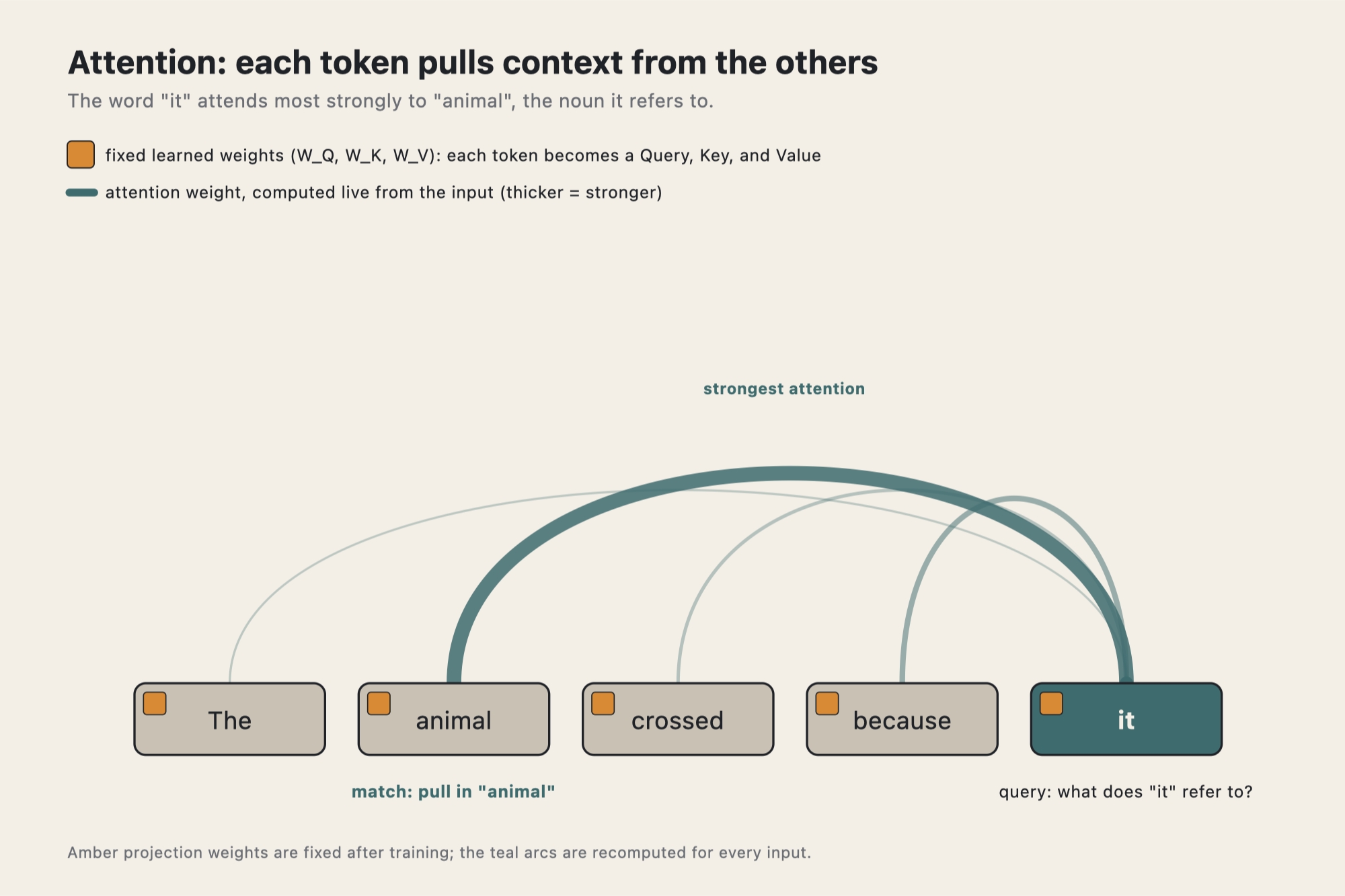
Everything up to this point processes each token on its own. But meaning depends on context. In the sentence "The animal didn't cross the street because it was too tired," the word "it" is useless until you know it refers to "animal." Attention is the mechanism that lets each token look at every other token and pull in what is relevant. It is the communication step, and it is the one place a model computes part of its own wiring on the fly.
Each token arrives as a vector. The layer holds three learned weight matrices and multiplies every token through each one to produce three vectors per token:
- Query (Q): what am I looking for?
- Key (K): what do I offer, what am I?
- Value (V): what will I hand over if you attend to me?
Same token, three projections, because it plays three roles: the seeker, the advertised label, and the payload. The mechanism then runs in five steps, for a sequence of tokens:
- Project each token through the Q, K, and V matrices.
- Score. For each token, compare its query against every token's key with a dot product. The result is high when two vectors align, so it measures how much one token should care about another.
- Scale and softmax the scores into positive numbers that sum to 1, so each token spreads a fixed budget of attention across all the others.
- Mix values. Each token's output is the weighted sum of every token's value, weighted by those scores. This is where context flows in.
- Project out through a final matrix back to the model's width.
Here is the payoff of the amber-teal split. Attention involves two different things both loosely called weights. The Q, K, V, and output matrices are learned parameters, fixed after training (amber). The attention scores, the "who attends to whom," are computed fresh from the input on every single pass (teal). The fixed matrices decide how to turn tokens into queries, keys, and values; the routing between these specific tokens is computed on the spot, not stored. That is exactly why a model handles a sentence it has never seen.
A few important refinements sit on top of this core:
- Heads. Rather than one comparison blending every kind of relationship, a layer runs many attention heads in parallel, each with its own slice of the Q/K/V matrices, each learning a different relationship: pronoun reference, subject-verb agreement, nearby words, long-range links. Each head is one independent attention channel.
- Causal masking. Because an LLM predicts the next token, a token must not peek at tokens that come after it. Future scores are set to negative infinity before the softmax, which turns them to zero, so each token attends only to itself and earlier tokens. That is what lets a model generate left to right.
- The KV cache. When generating one token at a time, the keys and values of earlier tokens do not change, so they are computed once and cached; each new token only attends against the stored keys and values instead of reprocessing the whole sequence. The cache is simply persisted activations, and it is the biggest single inference speedup, as well as what consumes memory as context grows.
- Grouped-query attention (GQA). Because that cache is large, modern models let several query heads share one key/value head, shrinking the cache several times over with little quality loss.
The full flow through one layer, then, is: attention (tokens communicate) then a residual add, then a feed-forward network of two big matrices and a nonlinearity (each token processes what it gathered) then another residual add. Stack dozens of these and you have the model. Every arrow is a matrix multiply against fixed weights, except the softmax routing, which is computed live.
Where weights live: GGUF vs safetensors
The finished weights have to be stored in a file, and there are two families of format, from two different worlds.
safetensors was created as a safe replacement for older Python "pickle" files, which could execute arbitrary code when loaded. It is pure data: a small header describing each tensor, then one raw blob of numbers. It is weights only, so a model is really a folder, with the tokenizer, config, and other pieces in sibling files. It is the native format of the GPU and PyTorch training-and-serving stack, and it keeps weights in real dtypes like FP16 and BF16.
GGUF comes from the local-inference world. It is self-contained: the weights, the full tokenizer, the chat template, the architecture settings, and the quantization details all live in one portable file. Hand someone one GGUF and they can run it. It is built around aggressive quantization and rich embedded metadata, and it is what local runners like Ollama and LM Studio load.
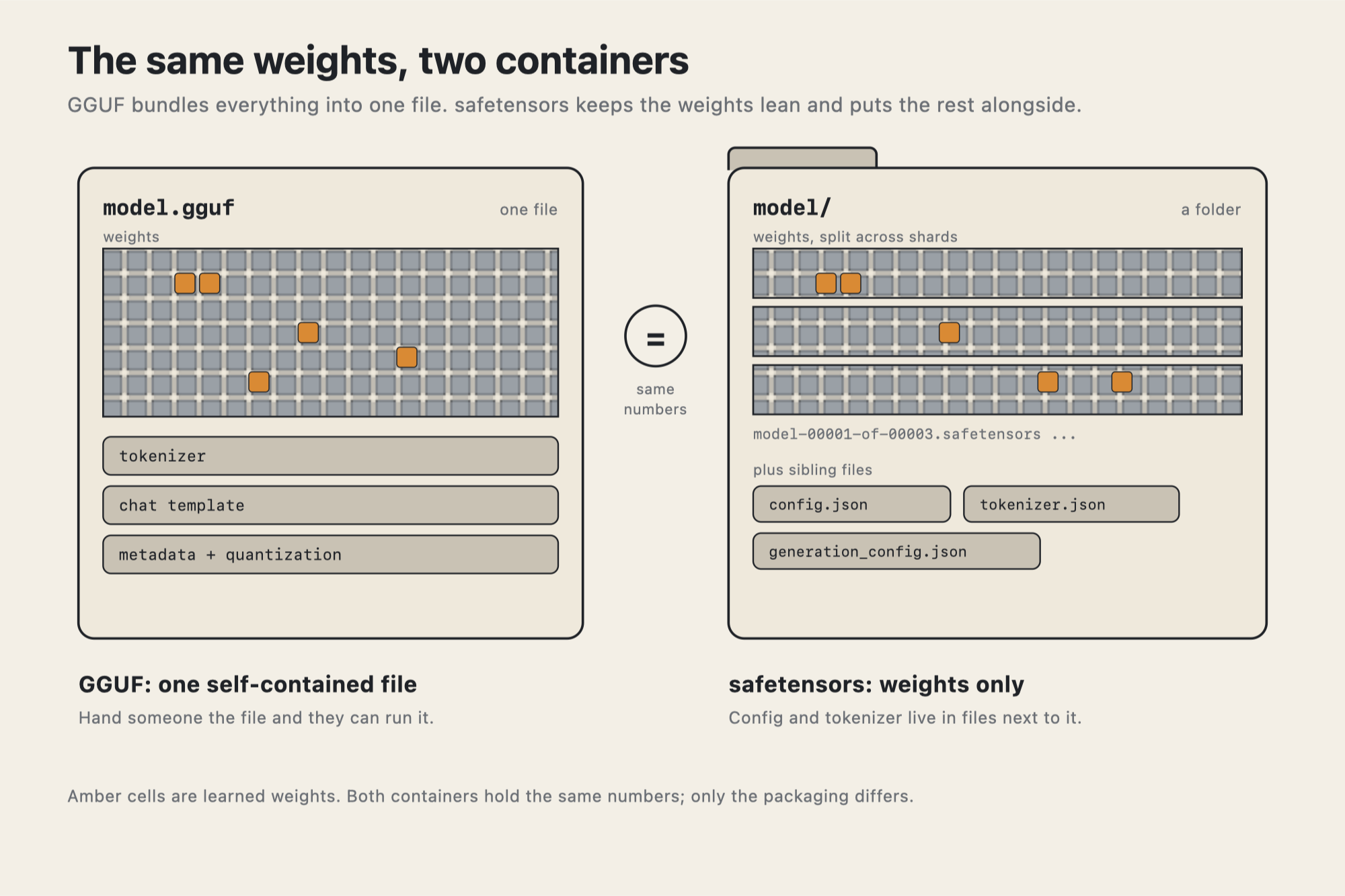
The split is an ecosystem difference, not a rivalry. Train and serve at scale on GPUs, and you use safetensors. Run a quantized model on your own machine, and you use GGUF. Which raises the obvious question: how does turning 16-bit weights into 4-bit ones not wreck the model?
Shrinking without breaking: quantization
Quantization is storing weights at fewer bits to save memory and speed. The surprise is that you can cut from 16 bits to 4, a fourfold reduction, and lose only a percent or two of quality. Three reasons why:
- The model was never using that precision. Knowledge is distributed and redundant across billions of weights; no single one is load-bearing. And the math is on your side: each layer output is a sum of thousands of weight-times-input products, rounding adds a small and roughly independent error to each, and the errors partially cancel. Signal grows with the number of terms while random noise grows only with its square root, so signal-to-noise actually improves with width. Wide matrices are more robust to rounding, not less.
- Inference is forgiving. This is the promise from the weights section, cashed in. Training compounds tiny errors over millions of steps; inference is a single forward pass with no accumulation. A little rounding stays a little rounding. You can serve at 4-bit and never train at 4-bit.
- Modern quantization is smart, not naive. Weights are split into small blocks, each with its own higher-precision scale, so one outlier can only distort its own block. Sensitive tensors are kept at higher bit-depth (this is what the
Q4_K_M-style suffixes encode). And calibration methods run sample data through the model and adjust the remaining weights to compensate for the rounding just introduced.
It does eventually break. Sixteen to eight bits is essentially free. Eight to four is the sweet spot, a couple of percent at most. Below four, quality falls off a cliff. One rule matters in practice: bigger models tolerate quantization better because they have more redundancy, so on a fixed memory budget a large model at 4-bit usually beats a small model at 16-bit. The payoff is that a 140GB model becomes a 40GB one that fits hardware it otherwise could not, and because inference is bound by how fast weights stream from memory, fewer bytes per weight also generates tokens faster.

Changing the weights: fine-tuning, LoRA, and QLoRA
Everything so far treats the weights as frozen after training. Fine-tuning is the one time they change again: continued training that starts from the pretrained weights instead of random ones, on a smaller, targeted dataset, to bend a general model toward a specific job.
Doing it the obvious way, unfreezing every weight, is brutally expensive, not because of the weights themselves but because of what training needs alongside them. Per parameter you must hold the weight, its gradient, and the optimizer's running averages, mostly in FP32, roughly 16 bytes each. For a 70-billion-parameter model that is over a terabyte of memory, a cluster rather than a single machine.
LoRA (Low-Rank Adaptation) rests on one observation: the change fine-tuning makes to a weight matrix is low-rank, so it can be approximated by the product of two skinny matrices. Instead of learning the full update, you learn those two small matrices and freeze the original weights entirely. For a 4096-by-4096 matrix, a rank-8 adapter is about 250 times fewer numbers. Because the expensive parts now scale with the tiny adapter rather than the whole model, single-GPU fine-tuning becomes possible; an adapter is a few megabytes rather than a full model copy, so one base model can hot-swap many of them; and the adapter can be merged back into the weights for zero cost at inference.
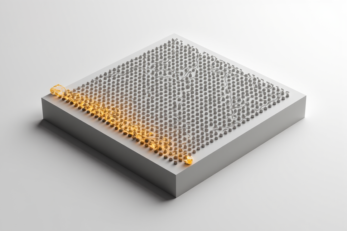
QLoRA combines this with quantization and closes the loop on the whole post. Load the base model frozen and quantized to 4-bit; since it is frozen, quantizing it is nearly free, exactly the inference-is-forgiving argument again. Then train the small LoRA adapters at higher precision on top. The result is that a 70-billion-parameter model can be fine-tuned on a single consumer-class GPU, something that used to require a cluster.
One last piece of judgment: fine-tuning is only one of three ways to change a model's behavior. Prompting changes the input, temporarily. Retrieval-augmented generation (RAG) adds retrieved context, and is the right tool for injecting facts. Fine-tuning changes the weights, permanently, and is the right tool for changing behavior, format, and style. The common mistake is fine-tuning to add facts; use retrieval for knowledge and fine-tuning for how the model should behave.
The whole picture in one paragraph
An LLM is a stack of Transformer layers whose weights (learned numbers, stored as quantizable low-precision values in a safetensors folder or a single GGUF file) are fixed matrices that data flows through as activations. Each layer's attention turns tokens into queries, keys, and values through fixed weight matrices, then routes information between tokens using scores computed live from the input, while a feed-forward stage lets each token process what it gathered. Training discovers the weights from data, slowly and precision-sensitively, in mixed BF16 and FP32. Inference replays them, forgivingly, quantized down to 4 bits for memory and speed. And fine-tuning, usually via LoRA or QLoRA over frozen quantized weights, bends the finished model toward a specific job by learning a tiny low-rank adjustment. Everything else is plumbing around those numbers.
That is the whole machine, from a single decimal to a fine-tuned model, with no term left pointing at another term you do not have.
---
Glossary
- Weights: the learned numbers inside a model, stored as matrices, that input is multiplied against to produce output.
- Training: the one-time, expensive process that discovers the weights by predicting tokens and nudging every number toward better guesses.
- Inference: running the finished model with frozen weights to generate output, one forward pass per token.
- dtype: the data type each weight is stored as, which sets its bit-width and precision (FP32, FP16, BF16, FP8, INT8, INT4).
- BF16: a 16-bit float that keeps FP32's full range and gives up precision, the modern training default.
- Mixed precision: training in fast BF16 while keeping a master copy of weights and optimizer state in FP32 so small updates accumulate faithfully.
- Tensor: a grid of numbers of any dimension: scalar (0-D), vector (1-D), matrix (2-D), or higher.
- Scalar: a single number, a 0-D tensor; a shape fact, not necessarily learned.
- Parameter: a number the training learned, a weight or bias; a role fact, always learned.
- Dims: a tensor's shape, or the model's width, how many numbers represent each token internally.
- Layer count: the depth of the model, how many Transformer blocks are stacked.
- Activations: the intermediate values that flow through the network on a given input, recomputed every forward pass.
- Activation function: the nonlinear function (ReLU, GELU, SiLU) applied after a matrix multiply so stacked layers do not collapse into one linear map.
- PyTorch: the framework most models are built and trained in, providing tensors, GPU math, and autograd.
- Transformer: the 2017 architecture every modern LLM uses, built around attention; also the name of a popular library.
- Attention: the step where each token looks at every other token in context and pulls in what is relevant.
- Q, K, V: Query, Key, and Value, three projections of each token produced by three fixed weight matrices.
- Attention head: one independent attention channel; a layer runs many in parallel, each learning a different relationship.
- Causal masking: setting future-token scores to negative infinity so each token attends only to itself and earlier tokens.
- KV cache: the stored keys and values of past tokens, reused each step so decoding does not reprocess the whole sequence.
- GQA: grouped-query attention, letting several query heads share one key/value head to shrink the KV cache.
- GPT: Generative Pre-trained Transformer, a naming convention for the approach nearly all modern LLMs follow.
- Hyperparameters: the human-chosen settings for the model and its training, as opposed to the learned weights.
- Tokenizer: the translator that encodes text into integer token ids and decodes model output ids back into text.
- Tokens: sub-word chunks the model reads instead of characters, roughly four characters or three-quarters of a word each in English.
- Chat template: the formatting rule that flattens conversation turns into the token string a model expects.
- safetensors: a safe, code-free weights container; weights only, with config and tokenizer in sibling files.
- GGUF: a self-contained single-file format holding weights, metadata, full tokenizer, chat template, and quantization info.
- Quantization: storing weights at fewer bits to shrink memory and speed inference, at a small quality cost.
- Fine-tuning: continued training from pretrained weights on a smaller targeted dataset to change behavior, format, or style.
- LoRA: approximating the fine-tuning update as two skinny matrices, training only those while the base weights stay frozen.
- QLoRA: LoRA over a base model frozen and quantized to 4-bit, which fits a large fine-tune on a single GPU.
- RAG: retrieval-augmented generation, adding retrieved context to inject facts, as opposed to changing weights.
Comments
// Comments are reviewed before appearing. No spam. No noise.